Sometimes you’re creating a Google Sheets spreadsheet for others to use, you can make it easier to refer to certain sections of data by renaming columns or rows using named ranges. Here’s how Rename Columns or Rows in Sheets.

Rename Columns or Rows in Google Sheets

Introduce

Google sheets is famous app for all uses want to fast edit online by Web service.

What Are Named Ranges?

Named ranges allow you to add a custom name to a group of cells, from entire columns or rows to smaller groups of cells. Creating a named range doesn’t overwrite the original cell references (A1, A2, etc.), but it does make it easier to refer to these cells (and the data contained within them) when you’re adding new formulas.

Using the Name Box

The quickest way to add a named range to Google Sheets is to use the name box. This is the box, positioned to the left of the formula bar, that shows you the cell reference for the cell or cells that are currently selected in your spreadsheet.

To begin, open your Google Sheets spreadsheet and select a new column or row. With the row or column selected, replace the existing cell reference in the name box with a new name, and then press the Enter key to save your choice.

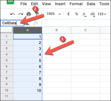
Google Sheets will apply the new name to your column or row immediately. You can view a list of existing named ranges by pressing the downward-facing arrow button positioned to the right of the name box.

A list of named ranges, including their original cell references, will appear in the list below.

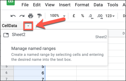
You can click on any of the named ranges to select those cells or press “Manage Named Ranges” to make changes to existing named ranges.

• Read more : How to Insert an Image in Google Sheets

Using the Named Ranges Menu

Another way to rename columns or rows is to use the named ranges menu. This menu allows you to manage existing named ranges as well as create new ones.

Adding a New Named Range in Google Sheets

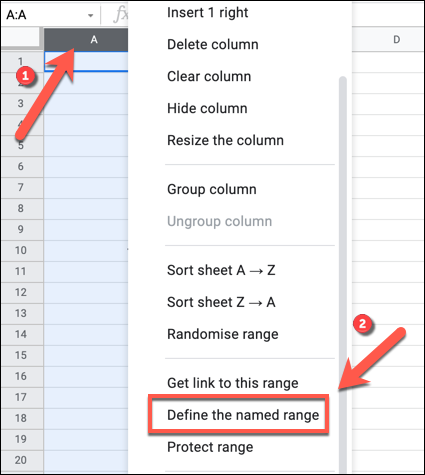
To begin, open Google Sheets and select the row or column that you wish to rename. With the column or row selected, right-click the selected cells and select “Define The Named Range” in the context menu.

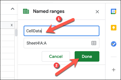
The “Named Ranges” menu will open as a panel on the right. Type your chosen name in the box provided. You can also change the selected column, row, or smaller cell range by changing the cell reference below it.

Press “Done” to save your choice.

Editing or Removing Named Ranges

To edit or remove a named range, right-click any cell in the spreadsheet and select “Define Named Range” in the menu. You’ll see a list of existing named ranges in a sidebar on the right side of the window. Hover over the name in the “Named Ranges” panel and press the “Edit” button.

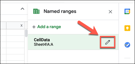
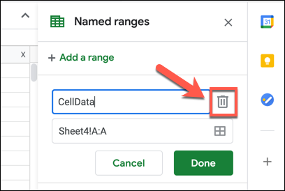
You can then make changes to the named range (including changing the name and the cell range that it refers to) using the boxes provided. If you want to delete the named range, press the “Delete” button.

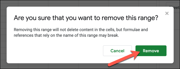
You’ll need to confirm your choice—press “Remove” in the pop-up box to confirm.

Using a Named Range in Google Sheets

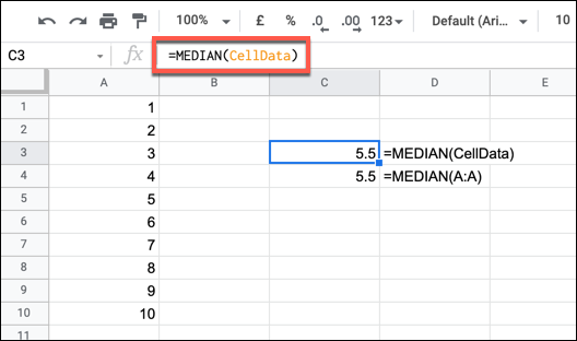
With the new named range added, you can now refer to it elsewhere in a new formula. For instance, if you named your range “CellData,” you could find the median value of the values in those cells by using the following formula:

The named range (CellData) replaces the original cell reference to the column, row, or cell range in your formula. For instance, if CellData is a named range for all of the cells in column A, you could use either A:A or CellData to refer to those cells.

Using a named range allows you to quickly refer to the data that you wish to use without requiring the original cell reference. It’s just one more way to use the power of Google Sheets to make things easier while you work.